A new benchmark runner for PyPy
The https://speed.pypy.org site has been running the PyPy benchmark suite since 2010. Our first benchmarking machine was called tannit, and it faithfully ran the suite from May 2010 to Dec 2016. For a brief period in the middle we had a machine called speed-python, but tannit was the gold standard. In June 2016 we started running benchmarks on our current machine, benchmarker (Intel i7-7700). It has been graciously sponsored by Baroque Software. Based on an Ubuntu xenial chroot, the machine has been quite stable but over the years has had a few kernel exploits blocked in firmware that changed its base performance.
It is time to update. Rather than use the same machine with updated software, we decided to opt for different hardware. Since the beginning of May we have been running the benchmark suite on benchmarker2: an AMD Ryzen 5 3600 machine. In order to try to stabilize benchmarks the machine was set up:
- without SMT (hyper-threading)
- using
cpusetto partition CPUs 3,4,5 off (the CPU has 2 CCD chiplets so the CPU sets are truly independent, the reason we chose the Zen2 architecture) and use them exclusively for benchmarking - disable turbo speed strategy.
It runs debian13 as a base operating system, and the benchmarks run in a
manylinux2_28 docker, which provides gcc14.
In order to establish a baseline, I compiled CPython 3.11.5 with:
./configure --prefix=/opt/cpython-3.11 --enable-optimizations \
--with-computed-gotos --enable-shared LDFLAGS='-Wl,-rpath,\$$ORIGIN/../lib'
The difference between the two machines is striking: where the xenial image (with GCC 5.4) benchmark comparison to CPython 3.11.9 shows a 3x improvement when run on PyPy on benchmarker, the newer machine with the newer compiler and a fresh baseline shows a 4.3x improvement. I can only speculate that the major differences between the results is:
- The CPython 3.11.9 run was done in June 2024. This was before some firmware kernel changes applied to the host machine that slowed it down. I did notice at the time the exploit migitagion firmware was applied that the overall comparison dropped from 3.3x to 3x, but felt the additional protection was warrented.
- The newer software image uses GCC 14, where the older one used GCC 5.
- The AMD machine has 32MB of L3 cache, the Intel machine has 8MB.
- The AMD machine uses RAM at 3200MHz, the Intel at 2400MHz.
The last 3 points may affect PyPy more than CPython, since PyPy's JIT is more memory intensive and the RPython codegen may be handled better by newer compilers.
This is the first step in an overhaul of PyPy's infrastructure. Other plans in the pipeline:
- Move all the buildbot builds from
manylinux_2014tomanylinux2_28-based images. This will match the move on benchmarker2. It will require some adaptations so that tests will pass on the newer compiler, see pypy/pypy#5488. This will mean an ABI break, so the next PyPy release will leave behind the 7.3.x series. - Think about updating our use of buildbot 0.8.8, which is woefully out of date. Since we have a heavily customized summary page, and the twistd-based endpoints are not supported on buildbot 0.9 and up, we set up a build-summary alternative that is synchronized to the buildbot work.
- Perhaps make more use of the free GitHub actions workers to replace or enhance the buildbot workers. Some of that can be seen in PR 5488. The build-summary service is also able to ingest github action testing results.
- Continue to push on in CPython compatibility, performance improvements, and bugfixes, as well as work on a PyPy 3.12 version
Help of course is welcome.
Matti
PyPy v7.3.23 release
PyPy v7.3.23: release of python 2.7, 3.11
The PyPy team is proud to release version 7.3.23 of PyPy after the previous release on April 26, 2026. This is a bug-fix release that fixes an overeager warning about unused coroutines, and some problems around multiple inheritance in c-extensions.
This version includes a change to the bytecode interpreter to use exception tables instead of dedicated opcodes. Now the PyPy disassembly will be closer to CPython format. So far it does not impact performance.
The release includes two different interpreters:
PyPy2.7, which is an interpreter supporting the syntax and the features of Python 2.7 including the stdlib for CPython 2.7.18+ (the
+is for backported security updates)PyPy3.11, which is an interpreter supporting the syntax and the features of Python 3.11, including the stdlib for CPython 3.11.15.
The interpreters are based on much the same codebase, thus the double release. This is a micro release, all APIs are compatible with the other 7.3 releases.
We recommend updating. You can find links to download the releases here:
We would like to thank our donors for the continued support of the PyPy project. If PyPy is not quite good enough for your needs, we are available for direct consulting work. If PyPy is helping you out, we would love to hear about it and encourage submissions to our blog via a pull request to https://github.com/pypy/pypy.org
We would also like to thank our contributors and encourage new people to join the project. PyPy has many layers and we need help with all of them: bug fixes, PyPy and RPython documentation improvements, or general help with making RPython's JIT even better.
If you are a python library maintainer and use C-extensions, please consider making a HPy / CFFI / cppyy version of your library that would be performant on PyPy. In any case, cibuildwheel supports building wheels for PyPy.
What is PyPy?
PyPy is a Python interpreter, a drop-in replacement for CPython. It's fast (PyPy and CPython performance comparison) due to its integrated tracing JIT compiler.
We also welcome developers of other dynamic languages to see what RPython can do for them.
We provide binary builds for:
x86 machines on most common operating systems (Linux 32/64 bits, Mac OS 64 bits, Windows 64 bits)
64-bit ARM machines running Linux (
aarch64) and macos (macos_arm64).
PyPy supports Windows 32-bit, Linux PPC64 big- and little-endian, Linux ARM 32 bit, RISC-V RV64IMAFD Linux, and s390x Linux but does not release binaries. Please reach out to us if you wish to sponsor binary releases for those platforms. Downstream packagers provide binary builds for debian, Fedora, conda, OpenBSD, FreeBSD, Gentoo, and more.
What else is new?
For more information about the 7.3.23 release, see the full changelog.
Please update, and continue to help us make pypy better.
Cheers, The PyPy Team
PyPy v7.3.22 release
PyPy v7.3.22: release of python 2.7, 3.11
The PyPy team is proud to release version 7.3.22 of PyPy after the previous release on March 13, 2026. This is a bug-fix release that fixes several issues in the JIT. Among them, a long-standing JIT bug that started appearing when some instance optimizations exposed it. We also cleaned up many of the remaining stdlib test suite failures, which improves CPython compatibility around line numbers in dis.dis, signatures and objclass attributes for builtins, and other quality of life features.
There is now an RPython _pickle module that mirrors
the CPython one, greatly speeding up pickling operations. Where before PyPy was
5.7x slower than CPython on the pickle benchmark from the pyperformance
benchmark suite, now it is only 1.6x slower [0]. We also added pypy
pickler extensions to dump and load lists using list strategies, and enabled
them in the ForkingPickler used by multiprocessing, speeding up cases where
such objects are passed between PyPy multiprocessing instances.
We also added an RPython json encoder, speeding up json_bench from being 2.6x slower than CPython to being 0.7x (meaning faster).
The release includes two different interpreters:
PyPy2.7, which is an interpreter supporting the syntax and the features of Python 2.7 including the stdlib for CPython 2.7.18+ (the
+is for backported security updates)PyPy3.11, which is an interpreter supporting the syntax and the features of Python 3.11, including the stdlib for CPython 3.11.15.
The interpreters are based on much the same codebase, thus the double release. This is a micro release, all APIs are compatible with the other 7.3 releases.
We recommend updating. You can find links to download the releases here:
We would like to thank our donors for the continued support of the PyPy project. If PyPy is not quite good enough for your needs, we are available for direct consulting work. If PyPy is helping you out, we would love to hear about it and encourage submissions to our blog via a pull request to https://github.com/pypy/pypy.org
We would also like to thank our contributors and encourage new people to join the project. PyPy has many layers and we need help with all of them: bug fixes, PyPy and RPython documentation improvements, or general help with making RPython's JIT even better.
If you are a python library maintainer and use C-extensions, please consider making a HPy / CFFI / cppyy version of your library that would be performant on PyPy. In any case, cibuildwheel supports building wheels for PyPy.
Footnotes
What is PyPy?
PyPy is a Python interpreter, a drop-in replacement for CPython It's fast (PyPy and CPython performance comparison) due to its integrated tracing JIT compiler.
We also welcome developers of other dynamic languages to see what RPython can do for them.
We provide binary builds for:
x86 machines on most common operating systems (Linux 32/64 bits, Mac OS 64 bits, Windows 64 bits)
64-bit ARM machines running Linux (
aarch64) and macos (macos_arm64).
PyPy supports Windows 32-bit, Linux PPC64 big- and little-endian, Linux ARM 32 bit, RISC-V RV64IMAFD Linux, and s390x Linux but does not release binaries. Please reach out to us if you wish to sponsor binary releases for those platforms. Downstream packagers provide binary builds for debian, Fedora, conda, OpenBSD, FreeBSD, Gentoo, and more.
What else is new?
For more information about the 7.3.22 release, see the full changelog.
Please update, and continue to help us make pypy better.
Cheers, The PyPy Team
Using Claude to fix PyPy3.11 test failures securely
I got access to Claude Max for 6 months, as a promotional move Anthropic made to Open Source Software contributors. My main OSS impact is as a maintainer for NumPy, but I decided to see what claude-code could to for PyPy's failing 3.11 tests. Most of these failures are edge cases: error messages that differ from CPython, or debugging tools that fail in certain cases. I was worried about letting an AI agent loose on my development machine. I noticed a post by Patrick McCanna (thanks Patrick!) that pointed to using bubblewrap to sandbox the agent. So I set it all up and (hopefully securely) pointed claude-code at some tests.
PyPy v7.3.21 release
PyPy v7.3.21: release of python 2.7, 3.11
The PyPy team is proud to release version 7.3.21 of PyPy after the previous release on July 4, 2025. This is a bug-fix release that also updates to Python 3.11.15.
The release includes two different interpreters:
PyPy2.7, which is an interpreter supporting the syntax and the features of Python 2.7 including the stdlib for CPython 2.7.18+ (the
+is for backported security updates)PyPy3.11, which is an interpreter supporting the syntax and the features of Python 3.11, including the stdlib for CPython 3.11.15.
The interpreters are based on much the same codebase, thus the double release. This is a micro release, all APIs are compatible with the other 7.3 releases.
We recommend updating. You can find links to download the releases here:
We would like to thank our donors for the continued support of the PyPy project. If PyPy is not quite good enough for your needs, we are available for direct consulting work. If PyPy is helping you out, we would love to hear about it and encourage submissions to our blog via a pull request to https://github.com/pypy/pypy.org
We would also like to thank our contributors and encourage new people to join the project. PyPy has many layers and we need help with all of them: bug fixes, PyPy and RPython documentation improvements, or general help with making RPython's JIT even better.
If you are a python library maintainer and use C-extensions, please consider making a HPy / CFFI / cppyy version of your library that would be performant on PyPy. In any case, cibuildwheel supports building wheels for PyPy.
What is PyPy?
PyPy is a Python interpreter, a drop-in replacement for CPython It's fast (PyPy and CPython performance comparison) due to its integrated tracing JIT compiler.
We also welcome developers of other dynamic languages to see what RPython can do for them.
We provide binary builds for:
x86 machines on most common operating systems (Linux 32/64 bits, Mac OS 64 bits, Windows 64 bits)
64-bit ARM machines running Linux (
aarch64) and macos (macos_arm64).
PyPy supports Windows 32-bit, Linux PPC64 big- and little-endian, Linux ARM 32 bit, RISC-V RV64IMAFD Linux, and s390x Linux but does not release binaries. Please reach out to us if you wish to sponsor binary releases for those platforms. Downstream packagers provide binary builds for debian, Fedora, conda, OpenBSD, FreeBSD, Gentoo, and more.
What else is new?
For more information about the 7.3.21 release, see the full changelog.
Please update, and continue to help us make pypy better.
Cheers, The PyPy Team
Load and store forwarding in the Toy Optimizer
This is a cross-post from Max Bernstein from his blog where he writes about programming languages, compilers, optimizations, virtual machines.
A long, long time ago (two years!) CF Bolz-Tereick and I made a video about load/store forwarding and an accompanying GitHub Gist about load/store forwarding (also called load elimination) in the Toy Optimizer. I said I would write a blog post about it, but never found the time—it got lost amid a sea of large life changes.
It's a neat idea: do an abstract interpretation over the trace, modeling the heap at compile-time, eliminating redundant loads and stores. That means it's possible to optimize traces like this:
v0 = ...
v1 = load(v0, 5)
v2 = store(v0, 6, 123)
v3 = load(v0, 6)
v4 = load(v0, 5)
v5 = do_something(v1, v3, v4)
into traces like this:
v0 = ...
v1 = load(v0, 5)
v2 = store(v0, 6, 123)
v5 = do_something(v1, 123, v1)
(where load(v0, 5) is equivalent to *(v0+5) in C syntax and store(v0, 6,
123) is equvialent to *(v0+6)=123 in C syntax)
This indicates that we were able to eliminate two redundant loads by keeping around information about previous loads and stores. Let's get to work making this possible.
The usual infrastructure
We'll start off with the usual infrastructure from the Toy Optimizer series: a very stringly-typed representation of a trace-based SSA IR and a union-find rewrite mechanism.
This means we can start writing some new optimization pass and our first test:
def optimize_load_store(bb: Block):
    opt_bb = Block()
    # TODO: copy an optimized version of bb into opt_bb
    return opt_bb

def test_two_loads():
    bb = Block()
    var0 = bb.getarg(0)
    var1 = bb.load(var0, 0)
    var2 = bb.load(var0, 0)
    bb.escape(var1)
    bb.escape(var2)
    opt_bb = optimize_load_store(bb)
    assert bb_to_str(opt_bb) == """\
var0 = getarg(0)
var1 = load(var0, 0)
var2 = escape(var1)
var3 = escape(var1)"""
This test is asserting that we can remove duplicate loads. Why load twice if we can cache the result? Let's make that happen.
Caching loads
To do this, we'll model the the heap at compile-time. When I say "model", I mean that we will have an imprecise but correct abstract representation of the heap: we don't (and can't) have knowledge of every value, but we can know for sure that some addresses have certain values.
For example, if we have observed a load from object O at offset 8 v0 =
load(O, 8), we know that the SSA value v0 is at heap[(O, 8)]. That sounds
tautological, but it's not. Future loads can make use of this information.
def get_num(op: Operation, index: int=1):
    assert isinstance(op.arg(index), Constant)
    return op.arg(index).value

def optimize_load_store(bb: Block):
    opt_bb = Block()
    # Stores things we know about the heap at... compile-time.
    # Key: an object and an offset pair acting as a heap address
    # Value: a previous SSA value we know exists at that address
    compile_time_heap: Dict[Tuple[Value, int], Value] = {}
    for op in bb:
        if op.name == "load":
            obj = op.arg(0)
            offset = get_num(op, 1)
            load_info = (obj, offset)
            previous = compile_time_heap.get(load_info)
            if previous is not None:
                op.make_equal_to(previous)
                continue
            compile_time_heap[load_info] = op
        opt_bb.append(op)
    return opt_bb
This pass records information about loads and uses the result of a previous cached load operation if available. We treat the pair of (SSA value, offset) as an address into our abstract heap.
That's great! If you run our simple test, it should now pass. But what happens if we store into that address before the second load? Oops...
def test_store_to_same_object_offset_invalidates_load():
    bb = Block()
    var0 = bb.getarg(0)
    var1 = bb.load(var0, 0)
    var2 = bb.store(var0, 0, 5)
    var3 = bb.load(var0, 0)
    bb.escape(var1)
    bb.escape(var3)
    opt_bb = optimize_load_store(bb)
    assert bb_to_str(opt_bb) == """\
var0 = getarg(0)
var1 = load(var0, 0)
var2 = store(var0, 0, 5)
var3 = load(var0, 0)
var4 = escape(var1)
var5 = escape(var3)"""
This test fails because we are incorrectly keeping around var1 in our
abstract heap. We need to get rid of it and not replace var3 with var1.
Invalidating cached loads
So it turns out we have to also model stores in order to cache loads correctly. One valid, albeit aggressive, way to do that is to throw away all the information we know at each store operation:
def optimize_load_store(bb: Block):
    opt_bb = Block()
    compile_time_heap: Dict[Tuple[Value, int], Value] = {}
    for op in bb:
        if op.name == "store":
            compile_time_heap.clear()
        elif op.name == "load":
            # ...
        opt_bb.append(op)
    return opt_bb
That makes our test pass—yay!—but at great cost. It means any store operation mucks up redundant loads. In our world where we frequently read from and write to objects, this is what we call a huge bummer.
For example, a store to offset 4 on some object should never interfere with a load from a different offset on the same object1. We should be able to keep our load from offset 0 cached here:
def test_store_to_same_object_different_offset_does_not_invalidate_load():
    bb = Block()
    var0 = bb.getarg(0)
    var1 = bb.load(var0, 0)
    var2 = bb.store(var0, 4, 5)
    var3 = bb.load(var0, 0)
    bb.escape(var1)
    bb.escape(var3)
    opt_bb = optimize_load_store(bb)
    assert bb_to_str(opt_bb) == """\
var0 = getarg(0)
var1 = load(var0, 0)
var2 = store(var0, 4, 5)
var3 = escape(var1)
var4 = escape(var1)"""
We could try instead checking if our specific (object, offset) pair is in the heap and only removing cached information about that offset and that object. That would definitely help!
def optimize_load_store(bb: Block):
    opt_bb = Block()
    compile_time_heap: Dict[Tuple[Value, int], Value] = {}
    for op in bb:
        if op.name == "store":
            load_info = (op.arg(0), get_num(op, 1))
            if load_info in compile_time_heap:
                del compile_time_heap[load_info]
        elif op.name == "load":
            # ...
        opt_bb.append(op)
    return opt_bb
It makes our test pass, too, which is great news.
Unfortunately, this runs into problems due to aliasing: it's entirely possible
that our compile-time heap could contain a pair (v0, 0) and a pair (v1, 0) where v0
and v1 are the same object (but not known to the optimizer). Then we might
run into a situation where we incorrectly cache loads because the optimizer
doesn't know our abstract addresses (v0, 0) and (v1, 0) are actually the
same pointer at run-time.
This means that we are breaking abstract interpretation rules: our abstract interpreter has to correctly model all possible outcomes at run-time. This means to me that we should instead pick some tactic in-between clearing all information (correct but over-eager) and clearing only exact matches of object+offset (incorrect).
The term that will help us here is called an alias class. It is a name for a way to efficiently partition objects in your abstract heap into completely disjoint sets. Writes to any object in one class never affect objects in another class.
Our very scrappy alias classes will be just based on the offset: each offset is a different alias class. If we write to any object at offset K, we have to invalidate all of our compile-time offset K knowledge—even if it's for another object. This is a nice middle ground, and it's possible because our (made up) object system guarantees that distinct objects do not overlap, and also that we are not writing out-of-bounds.2
So let's remove all of the entries from compile_time_heap where the offset
matches the offset in the current store:
def optimize_load_store(bb: Block):
    opt_bb = Block()
    compile_time_heap: Dict[Tuple[Value, int], Value] = {}
    for op in bb:
        if op.name == "store":
            offset = get_num(op, 1)
            compile_time_heap = {
                load_info: value
                for load_info, value in compile_time_heap.items()
                if load_info[1] != offset
            }
        elif op.name == "load":
            # ...
        opt_bb.append(op)
    return opt_bb
Great! Now our test passes.
This concludes the load optimization section of the post. We have modeled enough of loads and stores that we can eliminate redundant loads. Very cool. But we can go further.
Caching stores
Stores don't just invalidate information. They also give us new information!
Any time we see an operation of the form v1 = store(v0, 8, 5) we also learn
that load(v0, 8) == 5! Until it gets invalidated, anyway.
For example, in this test, we can eliminate the load from var0 at offset 0:
def test_load_after_store_removed():
    bb = Block()
    var0 = bb.getarg(0)
    bb.store(var0, 0, 5)
    var1 = bb.load(var0, 0)
    var2 = bb.load(var0, 1)
    bb.escape(var1)
    bb.escape(var2)
    opt_bb = optimize_load_store(bb)
    assert bb_to_str(opt_bb) == """\
var0 = getarg(0)
var1 = store(var0, 0, 5)
var2 = load(var0, 1)
var3 = escape(5)
var4 = escape(var2)"""
Making that work is thankfully not very hard; we need only add that new information to the compile-time heap after removing all the potentially-aliased info:
def optimize_load_store(bb: Block):
    opt_bb = Block()
    compile_time_heap: Dict[Tuple[Value, int], Value] = {}
    for op in bb:
        if op.name == "store":
            offset = get_num(op, 1)
            compile_time_heap = # ... as before ...
            obj = op.arg(0)
            new_value = op.arg(2)
            compile_time_heap[(obj, offset)] = new_value  # NEW!
        elif op.name == "load":
            # ...
        opt_bb.append(op)
    return opt_bb
This makes the test pass. It makes another test fail, but only because—oops—we now know more. You can delete the old test because the new test supersedes it.
Now, note that we are not removing the store. This is because we have nothing
in our optimizer that keeps track of what might have observed the side-effects
of the store. What if the object got escaped? Or someone did a load later on?
We would only be able to remove the store (continue) if we could guarantee it
was not observable.
In our current framework, this only happens in one case: someone is doing a store of the exact same value that already exists in our compile-time heap. That is, either the same constant, or the same SSA value. If we see this, then we can completely skip the second store instruction.
Here's a test case for that, where we have gained information from the load instruction that we can then use to get rid of the store instruction:
def test_load_then_store():
    bb = Block()
    arg1 = bb.getarg(0)
    var1 = bb.load(arg1, 0)
    bb.store(arg1, 0, var1)
    bb.escape(var1)
    opt_bb = optimize_load_store(bb)
    assert bb_to_str(opt_bb) == """\
var0 = getarg(0)
var1 = load(var0, 0)
var2 = escape(var1)"""
Let's make it pass. To do that, first we'll make an equality function that works for both constants and operations. Constants are equal if their values are equal, and operations are equal if they are the identical (by address/pointer) operation.
def eq_value(left: Value|None, right: Value) -> bool:
    if isinstance(left, Constant) and isinstance(right, Constant):
        return left.value == right.value
    return left is right
This is a partial equality: if two operations are not equal under eq_value,
it doesn't mean that they are different, only that we don't know that they are
the same.
Then, after that, we need only check if the current value in the compile-time
heap is the same as the value being stored in. If it is, wonderful. No need to
store. continue and don't append the operation to opt_bb:
def optimize_load_store(bb: Block):
    opt_bb = Block()
    compile_time_heap: Dict[Tuple[Value, int], Value] = {}
    for op in bb:
        if op.name == "store":
            obj = op.arg(0)
            offset = get_num(op, 1)
            store_info = (obj, offset)
            current_value = compile_time_heap.get(store_info)
            new_value = op.arg(2)
            if eq_value(current_value, new_value):  # NEW!
                continue
            compile_time_heap = # ... as before ...
            # ...
        elif op.name == "load":
            load_info = (op.arg(0), get_num(op, 1))
            if load_info in compile_time_heap:
                op.make_equal_to(compile_time_heap[load_info])
                continue
            compile_time_heap[load_info] = op
        opt_bb.append(op)
    return opt_bb
This makes our load-then-store pass and it also makes other tests pass too, like eliminating a store after another store!
def test_store_after_store():
    bb = Block()
    arg1 = bb.getarg(0)
    bb.store(arg1, 0, 5)
    bb.store(arg1, 0, 5)
    opt_bb = optimize_load_store(bb)
    assert bb_to_str(opt_bb) == """\
var0 = getarg(0)
var1 = store(var0, 0, 5)"""
Unfortunately, this only works if the values—constants or SSA values—are known to be the same. If we store different values, we can't optimize. In the live stream, we left this an exercise for the viewer:
@pytest.mark.xfail
def test_exercise_for_the_reader():
    bb = Block()
    arg0 = bb.getarg(0)
    var0 = bb.store(arg0, 0, 5)
    var1 = bb.store(arg0, 0, 7)
    var2 = bb.load(arg0, 0)
    bb.escape(var2)
    opt_bb = optimize_load_store(bb)
    assert bb_to_str(opt_bb) == """\
var0 = getarg(0)
var1 = store(var0, 0, 7)
var2 = escape(7)"""
We would only be able to optimize this away if we had some notion of a store being dead. In this case, that is a store in which the value is never read before being overwritten.
Removing dead stores
TODO, I suppose. I have not gotten this far yet. If I get around to it, I will come back and update the post.
In the real world
This small optimization pass may seem silly or fiddly—when would we ever see something like this in a real IR?—but it's pretty useful. Here's the Ruby code that got me thinking about it again some years later for ZJIT:
class C
  def initialize
    @a = 1
    @b = 2
    @c = 3
  end
end
CRuby has a shape system and ZJIT makes use of it, so we end up optimizing this code (if it's monomorphic) into a series of shape checks and stores. The HIR might end up looking something like the mess below, where I've annotated the shape guards (can be thought of as loads) and stores with asterisks:
fn initialize@tmp/init.rb:3:
# ...
bb2(v6:BasicObject):
  v10:Fixnum[1] = Const Value(1)
  v31:HeapBasicObject = GuardType v6, HeapBasicObject
* v32:HeapBasicObject = GuardShape v31, 0x400000
* StoreField v32, :@a@0x10, v10
  WriteBarrier v32, v10
  v35:CShape[0x40008e] = Const CShape(0x40008e)
* StoreField v32, :_shape_id@0x4, v35
  v16:Fixnum[2] = Const Value(2)
  v37:HeapBasicObject = GuardType v6, HeapBasicObject
* v38:HeapBasicObject = GuardShape v37, 0x40008e
* StoreField v38, :@b@0x18, v16
  WriteBarrier v38, v16
  v41:CShape[0x40008f] = Const CShape(0x40008f)
* StoreField v38, :_shape_id@0x4, v41
  v22:Fixnum[3] = Const Value(3)
  v43:HeapBasicObject = GuardType v6, HeapBasicObject
* v44:HeapBasicObject = GuardShape v43, 0x40008f
* StoreField v44, :@c@0x20, v22
  WriteBarrier v44, v22
  v47:CShape[0x400090] = Const CShape(0x400090)
* StoreField v44, :_shape_id@0x4, v47
  CheckInterrupts
  Return v22
If we had store-load forwarding in ZJIT, we could get rid of the intermediate
shape guards; they would know the shape from the previous StoreField
instruction. If we had dead store elimination, we could get rid of the
intermediate shape writes; they are never read. (And the repeated type guards
to check if it's a heap object still are just silly and need to get removed
eventually.)
This is on the roadmap and will make object initialization even faster than it is right now.
Wrapping up
Thanks for reading the text version of the video that CF and I made a while back. Now you know how to do load/store elimination on traces.
I think this does not need too much extra work to get it going on full CFGs; a block is pretty much the same as a trace, so you can do a block-local version without much fuss. If you want to go global, you need dominator information and gen-kill sets.
Maybe I will touch on this in a future post...
Thank you
Thank you to CF, who walked me through this live on a stream two years ago! This blog post wouldn't be possible without you.
-
In this toy optimizer example, we are assuming that all reads and writes are the same size and different offsets don't overlap at all. This is often the case for managed runtimes, where object fields are pointer-sized and all reads/writes are pointed aligned. ↩
-
We could do better. If we had type information, we could also use that to make alias classes. Writes to a List will never overlap with writes to a Map, for example. This requires your compiler to have strict aliasing—if you can freely cast between types, as in C, then this tactic goes out the window.
This is called Type-based alias analysis (PDF). ↩
PyPy v7.3.20 release
PyPy v7.3.20: release of python 2.7, 3.11
The PyPy team is proud to release version 7.3.20 of PyPy after the previous
release on Feb 26, 2025. The release fixes some subtle bugs in ctypes and
OrderedDict and makes PyPy3.11 compatible with an upcoming release of
Cython.
The release includes two different interpreters:
PyPy2.7, which is an interpreter supporting the syntax and the features of Python 2.7 including the stdlib for CPython 2.7.18+ (the
+is for backported security updates)PyPy3.11, which is an interpreter supporting the syntax and the features of Python 3.11, including the stdlib for CPython 3.11.13.
The interpreters are based on much the same codebase, thus the double release. This is a micro release, all APIs are compatible with the other 7.3 releases.
We recommend updating. You can find links to download the releases here:
We would like to thank our donors for the continued support of the PyPy project. If PyPy is not quite good enough for your needs, we are available for direct consulting work. If PyPy is helping you out, we would love to hear about it and encourage submissions to our blog via a pull request to https://github.com/pypy/pypy.org
We would also like to thank our contributors and encourage new people to join the project. PyPy has many layers and we need help with all of them: bug fixes, PyPy and RPython documentation improvements, or general help with making RPython's JIT even better.
If you are a python library maintainer and use C-extensions, please consider making a HPy / CFFI / cppyy version of your library that would be performant on PyPy. In any case, cibuildwheel supports building wheels for PyPy.
What is PyPy?
PyPy is a Python interpreter, a drop-in replacement for CPython It's fast (PyPy and CPython performance comparison) due to its integrated tracing JIT compiler.
We also welcome developers of other dynamic languages to see what RPython can do for them.
We provide binary builds for:
x86 machines on most common operating systems (Linux 32/64 bits, Mac OS 64 bits, Windows 64 bits)
64-bit ARM machines running Linux (
aarch64) and macos (macos_arm64).
PyPy supports Windows 32-bit, Linux PPC64 big- and little-endian, Linux ARM 32 bit, RISC-V RV64IMAFD Linux, and s390x Linux but does not release binaries. Please reach out to us if you wish to sponsor binary releases for those platforms. Downstream packagers provide binary builds for debian, Fedora, conda, OpenBSD, FreeBSD, Gentoo, and more.
What else is new?
For more information about the 7.3.20 release, see the full changelog.
Please update, and continue to help us make pypy better.
Cheers, The PyPy Team
How fast can the RPython GC allocate?
While working on a paper about allocation profiling in VMProf I got curious about how quickly the RPython GC can allocate an object. I wrote a small RPython benchmark program to get an idea of the order of magnitude.
The basic idea is to just allocate an instance in a tight loop:
class A(object):
    pass

def run(loops):
    # preliminary idea, see below
    for i in range(loops):
        a = A()
        a.i = i
The RPython type inference will find out that instances of A have a single
i field, which is an integer. In addition to that field, every RPython object
needs one word of GC meta-information. Therefore one instance of A needs 16
bytes on a 64-bit architecture.
However, measuring like this is not good enough, because the RPython static optimizer would remove the allocation since the object isn't used. But we can confuse the escape analysis sufficiently by always keeping two instances alive at the same time:
class A(object):
    pass

def run(loops):
    a = prev = None
    for i in range(loops):
        prev = a
        a = A()
        a.i = i
    print(prev, a) # print the instances at the end
(I confirmed that the allocation isn't being removed by looking at the C code that the RPython compiler generates from this.)
This is doing a little bit more work than needed, because of the a.i = i
instance attribute write. We can also (optionally) leave the field
uninitialized.
def run(initialize_field, loops):
    t1 = time.time()
    if initialize_field:
        a = prev = None
        for i in range(loops):
            prev = a
            a = A()
            a.i = i
        print(prev, a) # make sure always two objects are alive
    else:
        a = prev = None
        for i in range(loops):
            prev = a
            a = A()
        print(prev, a)
    t2 = time.time()
    print(t2 - t1, 's')
    object_size_in_words = 2 # GC header, one integer field
    mem = loops * 8 * object_size_in_words / 1024.0 / 1024.0 / 1024.0
    print(mem, 'GB')
    print(mem / (t2 - t1), 'GB/s')
Then we need to add some RPython scaffolding:
def main(argv):
    loops = int(argv[1])
    with_init = bool(int(argv[2]))
    if with_init:
        print("with initialization")
    else:
        print("without initialization")
    run(with_init, loops)
    return 0

def target(*args):
    return main
To build a binary:
pypy rpython/bin/rpython targetallocatealot.py
Which will turn the RPython code into C code and use a C compiler to turn that into a binary, containing both our code above as well as the RPython garbage collector.
Then we can run it (all results again from my AMD Ryzen 7 PRO 7840U, running Ubuntu Linux 24.04.2):
$ ./targetallocatealot-c 1000000000 0
without initialization
<A object at 0x7c71ad84cf60> <A object at 0x7c71ad84cf70>
0.433825 s
14.901161 GB
34.348322 GB/s
$ ./targetallocatealot-c 1000000000 1
with initialization
<A object at 0x71b41c82cf60> <A object at 0x71b41c82cf70>
0.501856 s
14.901161 GB
29.692100 GB/s
Let's compare it with the Boehm GC:
$ pypy rpython/bin/rpython --gc=boehm --output=targetallocatealot-c-boehm targetallocatealot.py
...
$ ./targetallocatealot-c-boehm 1000000000 0
without initialization
<A object at 0xffff8bd058a6e3af> <A object at 0xffff8bd058a6e3bf>
9.722585 s
14.901161 GB
1.532634 GB/s
$ ./targetallocatealot-c-boehm 1000000000 1
with initialization
<A object at 0xffff88e1132983af> <A object at 0xffff88e1132983bf>
9.684149 s
14.901161 GB
1.538717 GB/s
This is not a fair comparison, because the Boehm GC uses conservative stack scanning, therefore it cannot move objects, which requires much more complicated allocation.
Let's look at perf stats
We can use perf to get some statistics about the executions:
$ perf stat -e cache-references,cache-misses,cycles,instructions,branches,faults,migrations ./targetallocatealot-c 10000000000 0
without initialization
<A object at 0x7aa260e35980> <A object at 0x7aa260e35990>
4.301442 s
149.011612 GB
34.642245 GB/s

 Performance counter stats for './targetallocatealot-c 10000000000 0':

     7,244,117,828      cache-references
        23,446,661      cache-misses                     #    0.32% of all cache refs
    21,074,240,395      cycles
   110,116,790,943      instructions                     #    5.23  insn per cycle
    20,024,347,488      branches
             1,287      faults
                24      migrations

       4.303071693 seconds time elapsed

       4.297557000 seconds user
       0.003998000 seconds sys

$ perf stat -e cache-references,cache-misses,cycles,instructions,branches,faults,migrations ./targetallocatealot-c 10000000000 1
with initialization
<A object at 0x77ceb0235980> <A object at 0x77ceb0235990>
5.016772 s
149.011612 GB
29.702688 GB/s

 Performance counter stats for './targetallocatealot-c 10000000000 1':

     7,571,461,470      cache-references
       241,915,266      cache-misses                     #    3.20% of all cache refs
    24,503,497,532      cycles
   130,126,387,460      instructions                     #    5.31  insn per cycle
    20,026,280,693      branches
             1,285      faults
                21      migrations

       5.019444749 seconds time elapsed

       5.012924000 seconds user
       0.005999000 seconds sys
This is pretty cool, we can run this loop with >5 instructions per cycle. Every
allocation takes 110116790943 / 10000000000 ≈ 11 instructions and
21074240395 / 10000000000 ≈ 2.1 cycles, including the loop around it.
How often does the GC run?
The RPython GC queries the L2 cache size to determine the size of the nursery.
We can find out what it is by turning on PYPYLOG, selecting the proper logging
categories, and printing to stdout via :-:
$ PYPYLOG=gc-set-nursery-size,gc-hardware:- ./targetallocatealot-c 1 1
[f3e6970465723] {gc-set-nursery-size
nursery size: 270336
[f3e69704758f3] gc-set-nursery-size}
[f3e697047b9a1] {gc-hardware
L2cache = 1048576
[f3e69705ced19] gc-hardware}
[f3e69705d11b5] {gc-hardware
memtotal = 32274210816.000000
[f3e69705f4948] gc-hardware}
[f3e6970615f78] {gc-set-nursery-size
nursery size: 4194304
[f3e697061ecc0] gc-set-nursery-size}
with initialization
NULL <A object at 0x7fa7b1434020>
0.000008 s
0.000000 GB
0.001894 GB/s
So the nursery is 4 MiB. This means that when we allocate 14.9 GiB the GC needs to perform 10000000000 * 16 / 4194304 ≈ 38146 minor collections. Let's confirm that:
$ PYPYLOG=gc-minor:out ./targetallocatealot-c 10000000000 1
with initialization
w<A object at 0x7991e3835980> <A object at 0x7991e3835990>
5.315511 s
149.011612 GB
28.033356 GB/s
$ head out
[f3ee482f4cd97] {gc-minor
[f3ee482f53874] {gc-minor-walkroots
[f3ee482f54117] gc-minor-walkroots}
minor collect, total memory used: 0
number of pinned objects: 0
total size of surviving objects: 0
time taken: 0.000029
[f3ee482f67b7e] gc-minor}
[f3ee4838097c5] {gc-minor
[f3ee48380c945] {gc-minor-walkroots
$ grep "{gc-minor-walkroots" out | wc -l
38147
Each minor collection is very quick, because a minor collection is O(surviving objects), and in this program only one object survive each time (the other instance is in the process of being allocated). Also, the GC root shadow stack is only one entry, so walking that is super quick as well. The time the minor collections take is logged to the out file:
$ grep "time taken" out | tail
time taken: 0.000002
time taken: 0.000002
time taken: 0.000002
time taken: 0.000002
time taken: 0.000002
time taken: 0.000002
time taken: 0.000002
time taken: 0.000003
time taken: 0.000002
time taken: 0.000002
$ grep "time taken" out | grep -o "0.*" | numsum
0.0988160000000011
(This number is super approximate due to float formatting rounding.)
that means that 0.0988160000000011 / 5.315511 ≈ 2% of the time is spent in the GC.
What does the generated machine code look like?
The allocation fast path of the RPython GC is a simple bump pointer, in Python pseudo-code it would look roughly like this:
result = gc.nursery_free
# Move nursery_free pointer forward by totalsize
gc.nursery_free = result + totalsize
# Check if this allocation would exceed the nursery
if gc.nursery_free > gc.nursery_top:
    # If it does => collect the nursery and al
    result = collect_and_reserve(totalsize)
result.hdr = <GC flags and type id of A>
So we can disassemble the compiled binary targetallocatealot-c and try to
find the equivalent logic in machine code. I'm super bad at reading machine
code, but I tried to annotate what I think is the core loop (the version
without initializing the i field) below:
    ...
    cb68:   mov    %rbx,%rdi
    cb6b:   mov    %rdx,%rbx

    # initialize object header of object allocated in previous iteration
    cb6e:   movq   $0x4c8,(%rbx)

    # loop termination check
    cb75:   cmp    %rbp,%r12
    cb78:   je     ccb8

    # load nursery_free
    cb7e:   mov    0x33c13(%rip),%rdx

    # increment loop counter
    cb85:   add    $0x1,%rbp

    # add 16 (size of object) to nursery_free
    cb89:   lea    0x10(%rdx),%rax

    # compare nursery_top with new nursery_free
    cb8d:   cmp    %rax,0x33c24(%rip)

    # store new nursery_free
    cb94:   mov    %rax,0x33bfd(%rip)

    # if new nursery_free exceeds nursery_top, fall through to slow path, if not, start at top
    cb9b:   jae    cb68

    # slow path from here on:
    # save live object from last iteration to GC shadow stack
    cb9d:   mov    %rbx,-0x8(%rcx)
    cba1:   mov    %r13,%rdi
    cba4:   mov    $0x10,%esi
    # do minor collection
    cba9:   call   20800 <pypy_g_IncrementalMiniMarkGC_collect_and_reserve>
    ...
Running the benchmark as regular Python code
So far we ran this code as RPython, i.e. type inference is performed and the program is translated to a C binary. We can also run it on top of PyPy, as a regular Python3 program. However, an instance of a user-defined class in regular Python when run on PyPy is actually a much larger object, due to dynamic typing. It's at least 7 words, which is 56 bytes.
However, we can simply use int objects instead. Integers are allocated on the
heap and consist of two words, one for the GC and one with the
machine-word-sized integer value, if the integer fits into a signed 64-bit
representation (otherwise a less compact different representation is used,
which can represent arbitrarily large integers).
Therefore, we can simply use this kind of code:
import sys, time


def run(loops):
    t1 = time.time()
    a = prev = None
    for i in range(loops):
        prev = a
        a = i
    print(prev, a) # make sure always two objects are alive
    t2 = time.time()
    object_size_in_words = 2 # GC header, one integer field
    mem = loops * 28 / 1024.0 / 1024.0 / 1024.0
    print(mem, 'GB')
    print(mem / (t2 - t1), 'GB/s')

def main(argv):
    loops = int(argv[1])
    run(loops)
    return 0

if __name__ == '__main__':
    sys.exit(main(sys.argv))
In this case we can't really leave the value uninitialized though.
We can run this both with and without the JIT:
$ pypy3 allocatealot.py 1000000000
999999998 999999999
14.901161193847656 GB
17.857494904899553 GB/s
$ pypy3 --jit off allocatealot.py 1000000000
999999998 999999999
14.901161193847656 GB
0.8275382375297171 GB/s
This is obviously much less efficient than the C code, the PyPy JIT generates much less efficient machine code than GCC. Still, "only" twice as slow is kind of cool anyway.
(Running it with CPython doesn't really make sense for this measurements, since
CPython ints are bigger – sys.getsizeof(5) reports 28 bytes.)
The machine code that the JIT generates
Unfortunately it's a bit of a journey to show the machine code that PyPy's JIT generates for this. First we need to run with all jit logging categories:
$ PYPYLOG=jit:out pypy3 allocatealot.py 1000000000
Then we can read the log file to find the trace IR for the loop under the logging category jit-log-opt:
+532: label(p0, p1, p6, p9, p11, i34, p13, p19, p21, p23, p25, p29, p31, i44, i35, descr=TargetToken(137358545605472))
debug_merge_point(0, 0, 'run;/home/cfbolz/projects/gitpypy/allocatealot.py:6-9~#24 FOR_ITER')

# are we at the end of the loop
+552: i45 = int_lt(i44, i35)
+555: guard_true(i45, descr=<Guard0x7ced4756a160>) [p0, p6, p9, p11, p13, p19, p21, p23, p25, p29, p31, p1, i44, i35, i34]
+561: i47 = int_add(i44, 1)
debug_merge_point(0, 0, 'run;/home/cfbolz/projects/gitpypy/allocatealot.py:6-9~#26 STORE_FAST')
debug_merge_point(0, 0, 'run;/home/cfbolz/projects/gitpypy/allocatealot.py:6-10~#28 LOAD_FAST')
debug_merge_point(0, 0, 'run;/home/cfbolz/projects/gitpypy/allocatealot.py:6-10~#30 STORE_FAST')
debug_merge_point(0, 0, 'run;/home/cfbolz/projects/gitpypy/allocatealot.py:6-11~#32 LOAD_FAST')
debug_merge_point(0, 0, 'run;/home/cfbolz/projects/gitpypy/allocatealot.py:6-11~#34 STORE_FAST')
debug_merge_point(0, 0, 'run;/home/cfbolz/projects/gitpypy/allocatealot.py:6-11~#36 JUMP_ABSOLUTE')

# update iterator object
+565: setfield_gc(p25, i47, descr=<FieldS pypy.module.__builtin__.functional.W_IntRangeIterator.inst_current 8>)
+569: guard_not_invalidated(descr=<Guard0x7ced4756a1b0>) [p0, p6, p9, p11, p19, p21, p23, p25, p29, p31, p1, i44, i34]

# check for signals
+569: i49 = getfield_raw_i(137358624889824, descr=<FieldS pypysig_long_struct_inner.c_value 0>)
+582: i51 = int_lt(i49, 0)
+586: guard_false(i51, descr=<Guard0x7ced4754db78>) [p0, p6, p9, p11, p19, p21, p23, p25, p29, p31, p1, i44, i34]
debug_merge_point(0, 0, 'run;/home/cfbolz/projects/gitpypy/allocatealot.py:6-9~#24 FOR_ITER')

# allocate the integer (allocation sunk to the end of the trace)
+592: p52 = new_with_vtable(descr=<SizeDescr 16>)
+630: setfield_gc(p52, i34, descr=<FieldS pypy.objspace.std.intobject.W_IntObject.inst_intval 8 pure>)
+634: jump(p0, p1, p6, p9, p11, i44, p52, p19, p21, p23, p25, p29, p31, i47, i35, descr=TargetToken(137358545605472))
To find the machine code address of the trace, we need to search for this line:
Loop 1 (run;/home/cfbolz/projects/gitpypy/allocatealot.py:6-9~#24 FOR_ITER) \
    has address 0x7ced473ffa0b to 0x7ced473ffbb0 (bootstrap 0x7ced473ff980)
Then we can use a script in the PyPy repo to disassemble the generated machine code:
$ pypy rpython/jit/backend/tool/viewcode.py out
This will dump all the machine code to stdout, and open a pygame-based graphviz cfg. In there we can search for the address and see this:
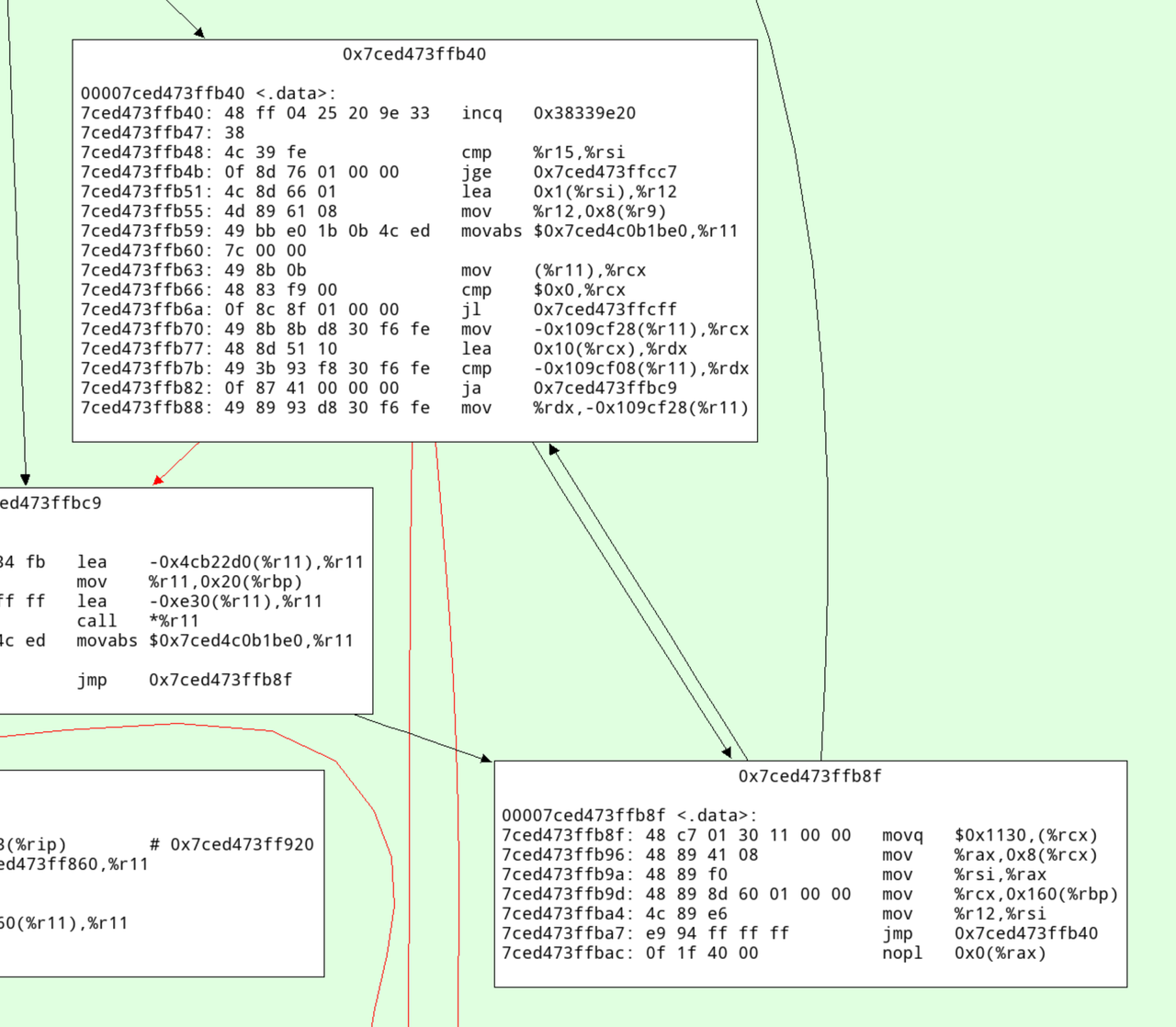
Here's an annotated version with what I think this code does:
# increment the profile counter
7ced473ffb40:   48 ff 04 25 20 9e 33    incq   0x38339e20
7ced473ffb47:   38

# check whether the loop is done
7ced473ffb48:   4c 39 fe                cmp    %r15,%rsi
7ced473ffb4b:   0f 8d 76 01 00 00       jge    0x7ced473ffcc7

# increment iteration variable
7ced473ffb51:   4c 8d 66 01             lea    0x1(%rsi),%r12

# update iterator object
7ced473ffb55:   4d 89 61 08             mov    %r12,0x8(%r9)

# check for ctrl-c/thread switch
7ced473ffb59:   49 bb e0 1b 0b 4c ed    movabs $0x7ced4c0b1be0,%r11
7ced473ffb60:   7c 00 00
7ced473ffb63:   49 8b 0b                mov    (%r11),%rcx
7ced473ffb66:   48 83 f9 00             cmp    $0x0,%rcx
7ced473ffb6a:   0f 8c 8f 01 00 00       jl     0x7ced473ffcff

# load nursery_free pointer
7ced473ffb70:   49 8b 8b d8 30 f6 fe    mov    -0x109cf28(%r11),%rcx

# add size (16)
7ced473ffb77:   48 8d 51 10             lea    0x10(%rcx),%rdx

# compare against nursery top
7ced473ffb7b:   49 3b 93 f8 30 f6 fe    cmp    -0x109cf08(%r11),%rdx

# jump to slow path if nursery is full
7ced473ffb82:   0f 87 41 00 00 00       ja     0x7ced473ffbc9

# store new value of nursery free
7ced473ffb88:   49 89 93 d8 30 f6 fe    mov    %rdx,-0x109cf28(%r11)

# initialize GC header
7ced473ffb8f:   48 c7 01 30 11 00 00    movq   $0x1130,(%rcx)

# initialize integer field
7ced473ffb96:   48 89 41 08             mov    %rax,0x8(%rcx)
7ced473ffb9a:   48 89 f0                mov    %rsi,%rax
7ced473ffb9d:   48 89 8d 60 01 00 00    mov    %rcx,0x160(%rbp)
7ced473ffba4:   4c 89 e6                mov    %r12,%rsi
7ced473ffba7:   e9 94 ff ff ff          jmp    0x7ced473ffb40
7ced473ffbac:   0f 1f 40 00             nopl   0x0(%rax)
Conclusion
The careful design of the RPython GC's allocation fast path gives pretty good allocation rates. This technique isn't really new, it's a pretty typical way to design a GC. Apart from that, my main conclusion would be that computers are fast or something? Indeed, when we ran the same code on my colleague's two-year-old AMD, we got quite a bit worse results, so a lot of the speed seems to be due to the hard work of CPU architects.
Doing the Prospero-Challenge in RPython
Recently I had a lot of fun playing with the Prospero Challenge by Matt Keeter. The challenge is to render a 1024x1024 image of a quote from The Tempest by Shakespeare. The input is a mathematical formula with 7866 operations, which is evaluated once per pixel.
What made the challenge particularly enticing for me personally was the fact that the formula is basically a trace in SSA-form – a linear sequence of operations, where every variable is assigned exactly once. The challenge is to evaluate the formula as fast as possible. I tried a number of ideas how to speed up execution and will talk about them in this somewhat meandering post. Most of it follows Matt's implementation Fidget very closely. There are two points of difference:
- I tried to add more peephole optimizations, but they didn't end up helping much.
- I implemented a "demanded information" optimization that removes a lot of operations by only keeping the sign of the result. This optimization ended up being useful.
Most of the prototyping in this post was done in RPython (a statically typable subset of Python2, that can be compiled to C), but I later rewrote the program in C to get better performance. All the code can be found on Github.
Input program
The input program is a sequence of operations, like this:
_0 const 2.95
_1 var-x
_2 const 8.13008
_3 mul _1 _2
_4 add _0 _3
_5 const 3.675
_6 add _5 _3
_7 neg _6
_8 max _4 _7
...
The first column is the name of the result variable, the second column is the
operation, and the rest are the arguments to the operation. var-x is a
special operation that returns the x-coordinate of the pixel being rendered,
and equivalently for var-y the y-coordinate. The sign of the result gives the
color of the pixel, the absolute value is not important.
A baseline interpreter
To run the program, I first parse them and replace the register names with indexes, to avoid any dictionary lookups at runtime. Then I implemented a simple interpreter for the SSA-form input program. The interpreter is a simple register machine, where every operation is executed in order. The result of the operation is stored into a list of results, and the next operation is executed. This was the slow baseline implementation of the interpreter but it's very useful to compare against the optimized versions.
This is roughly what the code looks like
class DirectFrame(object):
    def __init__(self, program):
        self.program = program
        self.next = None

    def run_floats(self, x, y, z):
        self.setxyz(x, y, z)
        return self.run()

    def setxyz(self, x, y, z):
        self.x = x
        self.y = y
        self.z = z

    def run(self):
        program = self.program
        num_ops = program.num_operations()
        floatvalues = [0.0] * num_ops
        for op in range(num_ops):
            func, arg0, arg1 = program.get_func_and_args(op)
            if func == OPS.const:
                floatvalues[op] = program.consts[arg0]
                continue
            farg0 = floatvalues[arg0]
            farg1 = floatvalues[arg1]
            if func == OPS.var_x:
                res = self.x
            elif func == OPS.var_y:
                res = self.y
            elif func == OPS.var_z:
                res = self.z
            elif func == OPS.add:
                res = self.add(farg0, farg1)
            elif func == OPS.sub:
                res = self.sub(farg0, farg1)
            elif func == OPS.mul:
                res = self.mul(farg0, farg1)
            elif func == OPS.max:
                res = self.max(farg0, farg1)
            elif func == OPS.min:
                res = self.min(farg0, farg1)
            elif func == OPS.square:
                res = self.square(farg0)
            elif func == OPS.sqrt:
                res = self.sqrt(farg0)
            elif func == OPS.exp:
                res = self.exp(farg0)
            elif func == OPS.neg:
                res = self.neg(farg0)
            elif func == OPS.abs:
                res = self.abs(farg0)
            else:
                assert 0
            floatvalues[op] = res
        return self.floatvalues[num_ops - 1]

    def add(self, arg0, arg1):
        return arg0 + arg1

    def sub(self, arg0, arg1):
        return arg0 - arg1

    def mul(self, arg0, arg1):
        return arg0 * arg1

    def max(self, arg0, arg1):
        return max(arg0, arg1)

    def min(self, arg0, arg1):
        return min(arg0, arg1)

    def square(self, arg0):
        val = arg0
        return val*val

    def sqrt(self, arg0):
        return math.sqrt(arg0)

    def exp(self, arg0):
        return math.exp(arg0)

    def neg(self, arg0):
        return -arg0

    def abs(self, arg0):
        return abs(arg0)
Running the naive interpreter on the prospero image file is super slow, since it performs 7866 * 1024 * 1024 float operations, plus the interpretation overhead.
Using Quadtrees to render the picture
The approach that Matt describes in his really excellent talk is to use quadtrees: recursively subdivide the image into quadrants, and evaluate the formula in each quadrant. For every quadrant you can simplify the formula by doing a range analysis. After a few recursion steps, the formula becomes significantly smaller, often only a few hundred or a few dozen operations.
At the bottom of the recursion you either reach a square where the range analysis reveals that the sign for all pixels is determined, then you can fill in all the pixels of the quadrant. Or you can evaluate the (now much simpler) formula in the quadrant by executing it for every pixel.
This is an interesting use case of JIT compiler/optimization techniques, requiring the optimizer itself to execute really quickly since it is an essential part of the performance of the algorithm. The optimizer runs literally hundreds of times to render a single image. If the algorithm is used for 3D models it becomes even more crucial.
Writing a simple optimizer
Implementing the quadtree recursion is straightforward. Since the program has no control flow the optimizer is very simple to write. I've written a couple of blog posts on how to easily write optimizers for linear sequences of operations, and I'm using the approach described in these Toy Optimizer posts. The interval analysis is basically an abstract interpretation of the operations. The optimizer does a sequential forward pass over the input program. For every operation, the output interval is computed. The optimizer also performs optimizations based on the computed intervals, which helps in reducing the number of operations executed (I'll talk about this further down).
Here's a sketch of the Python code that does the optimization:
class Optimizer(object):
    def __init__(self, program):
        self.program = program
        num_operations = program.num_operations()
        self.resultops = ProgramBuilder(num_operations)
        self.intervalframe = IntervalFrame(self.program)
        # old index -> new index
        self.opreplacements = [0] * num_operations
        self.index = 0

    def get_replacement(self, op):
        return self.opreplacements[op]

    def newop(self, func, arg0=0, arg1=0):
        return self.resultops.add_op(func, arg0, arg1)

    def newconst(self, value):
        const = self.resultops.add_const(value)
        self.intervalframe.minvalues[const] = value
        self.intervalframe.maxvalues[const] = value
        #self.seen_consts[value] = const
        return const

    def optimize(self, a, b, c, d, e, f):
        program = self.program
        self.intervalframe.setxyz(a, b, c, d, e, f)
        numops = program.num_operations()
        for index in range(numops):
            newop = self._optimize_op(index)
            self.opreplacements[index] = newop
        return self.opreplacements[numops - 1]

    def _optimize_op(self, op):
        program = self.program
        intervalframe = self.intervalframe
        func, arg0, arg1 = program.get_func_and_args(op)
        assert arg0 >= 0
        assert arg1 >= 0
        if func == OPS.var_x:
            minimum = intervalframe.minx
            maximum = intervalframe.maxx
            return self.opt_default(OPS.var_x, minimum, maximum)
        if func == OPS.var_y:
            minimum = intervalframe.miny
            maximum = intervalframe.maxy
            return self.opt_default(OPS.var_y, minimum, maximum)
        if func == OPS.var_z:
            minimum = intervalframe.minz
            maximum = intervalframe.maxz
            return self.opt_default(OPS.var_z, minimum, maximum)
        if func == OPS.const:
            const = program.consts[arg0]
            return self.newconst(const)
        arg0 = self.get_replacement(arg0)
        arg1 = self.get_replacement(arg1)
        assert arg0 >= 0
        assert arg1 >= 0
        arg0minimum = intervalframe.minvalues[arg0]
        arg0maximum = intervalframe.maxvalues[arg0]
        arg1minimum = intervalframe.minvalues[arg1]
        arg1maximum = intervalframe.maxvalues[arg1]
        if func == OPS.neg:
            return self.opt_neg(arg0, arg0minimum, arg0maximum)
        if func == OPS.min:
            return self.opt_min(arg0, arg1, arg0minimum, arg0maximum, arg1minimum, arg1maximum)
        ...

    def opt_default(self, func, minimum, maximum, arg0=0, arg1=0):
        self.intervalframe._set(newop, minimum, maximum)
        return newop

    def opt_neg(self, arg0, arg0minimum, arg0maximum):
        # peephole rules go here, see below
        minimum, maximum = self.intervalframe._neg(arg0minimum, arg0maximum)
        return self.opt_default(OPS.neg, minimum, maximum, arg0)

    @symmetric
    def opt_min(self, arg0, arg1, arg0minimum, arg0maximum, arg1minimum, arg1maximum):
        # peephole rules go here, see below
        minimum, maximum = self.intervalframe._max(arg0minimum, arg0maximum, arg1minimum, arg1maximum)
        return self.opt_default(OPS.max, minimum, maximum, arg0, arg1)

    ...
The resulting optimized traces are then simply interpreted at the bottom of the quadtree recursion. Matt talks about also generating machine code from them, but when I tried to use PyPy's JIT for that it was way too slow at producing machine code.
Testing soundness of the interval abstract domain
To make sure that my interval computation in the optimizer is correct, I implemented a hypothesis-based property based test. It checks the abstract transfer functions of the interval domain for soundness. It does so by generating random concrete input values for an operation and random intervals that surround the random concrete values, then performs the concrete operation to get the concrete output, and finally checks that the abstract transfer function applied to the input intervals gives an interval that contains the concrete output.
For example, the random test for the square operation would look like this:
from hypothesis import given, strategies, assume
from pyfidget.vm import IntervalFrame, DirectFrame
import math

regular_floats = strategies.floats(allow_nan=False, allow_infinity=False)

def make_range_and_contained_float(a, b, c):
    a, b, c, = sorted([a, b, c])
    return a, b, c

frame = DirectFrame(None)
intervalframe = IntervalFrame(None)

range_and_contained_float = strategies.builds(make_range_and_contained_float, regular_floats, regular_floats, regular_floats)

def contains(res, rmin, rmax):
    if math.isnan(rmin) or math.isnan(rmax):
        return True
    return rmin <= res <= rmax


@given(range_and_contained_float)
def test_square(val):
    a, b, c = val
    rmin, rmax = intervalframe._square(a, c)
    res = frame.square(b)
    assert contains(res, rmin, rmax)
This test generates a random float b, and two other floats a and c such
that the interval [a, c] contains b. The test then checks that the result
of the square operation on b is contained in the interval [rmin, rmax]
returned by the abstract transfer function for the square operation.
Peephole rewrites
The only optimization that Matt does in his implementation is a peephole
optimization rule that removes min and max operations where the intervals
of the arguments don't overlap. In that case, the optimizer statically can know
which of the arguments will be the result of the operation. I implemented this
peephole optimization in my implementation as well, but I also added a few more
peephole optimizations that I thought would be useful.
class Optimizer(object):

    def opt_neg(self, arg0, arg0minimum, arg0maximum):
        # new: add peephole rule --x => x
        func, arg0arg0, _ = self.resultops.get_func_and_args(arg0)
        if func == OPS.neg:
            return arg0arg0
        minimum, maximum = self.intervalframe._neg(arg0minimum, arg0maximum)
        return self.opt_default(OPS.neg, minimum, maximum, arg0)

    @symmetric
    def opt_min(self, arg0, arg1, arg0minimum, arg0maximum, arg1minimum, arg1maximum):
        # Matt's peephole rule
        if arg0maximum < arg1minimum:
            return arg0 # we can use the intervals to decide which argument will be returned
        # new one by me: min(x, x) => x
        if arg0 == arg1:
            return arg0
        func, arg0arg0, arg0arg1 = self.resultops.get_func_and_args(arg0)
        minimum, maximum = self.intervalframe._max(arg0minimum, arg0maximum, arg1minimum, arg1maximum)
        return self.opt_default(OPS.max, minimum, maximum, arg0, arg1)

    ...
However, it turns out that all my attempts at adding other peephole
optimization rules were not very useful. Most rules never fired, and the ones
that did only had a small effect on the performance of the program. The only
peephole optimization that I found to be useful was the one that Matt describes
in his talk. Matt's min/max optimization were 96% of all rewrites that my
peephole optimizer applied for the prospero.vm input. The remaining 4% of
rewrites were (the percentages are of that 4%):
--x => x                          4.65%
(-x)**2 => x ** 2                 0.99%
min(x, x) => x                   20.86%
min(x, min(x, y)) =>  min(x, y)  52.87%
max(x, x) => x                   16.40%
max(x, max(x, y)) => max(x, y)    4.23%
In the end it turned out that having these extra optimization rules made the total runtime of the system go up. Checking for the rewrites isn't free, and since they apply so rarely they don't pay for their own cost in terms of improved performance.
There are some further rules that I tried that never fired at all:
a * 0 => 0
a * 1 => a
a * a => a ** 2
a * -1 => -a
a + 0 => a
a - 0 => a
x - x => 0
abs(known positive number x) => x
abs(known negative number x) => -x
abs(-x) => abs(x)
(-x) ** 2 => x ** 2
This investigation is clearly way too focused on a single program and should be re-done with a larger set of example inputs, if this were an actually serious implementation.
Demanded Information Optimization
LLVM has an static analysis pass called 'demanded bits'. It is a backwards analysis that allows you to determine which bits of a value are actually used in the final result. This information can then be used in peephole optimizations. For example, if you have an expression that computes a value, but only the last byte of that value is used in the final result, you can optimize the expression to only compute the last byte.
Here's an example. Let's say we first byte-swap a 64-bit int, and then mask off the last byte:
uint64_t byteswap_then_mask(uint64_t a) {
    return byteswap(a) & 0xff;
}
In this case, the "demanded bits" of the byteswap(a) expression are
0b0...011111111, which inversely means that we don't care about the upper 56
bits. Therefore the whole expression can be optimized to a >> 56.
For the Prospero challenge, we can observe that for the resulting pixel values, the value of
the result is not used at all, only its sign. Essentially, every program ends
implicitly with a sign operation that returns 0.0 for negative values and
1.0 for positive values. For clarity, I will show this sign operation in
the rest of the section, even if it's not actually in the real code.
This makes it possible to simplify certain min/max operations further. Here is an example of a program, together with the intervals of the variables:
x var-x     # [0.1, 1]
y var-y     # [-1, 1]
m min x y # [-1, 1]
out sign m
This program can be optimized to:
y var-y
out sign m
Because that expression has the same result as the original expression: if x >
0.1, for the result of min(x, y) to be negative then y needs to be negative.
Another, more complex, example is this:
x var-x        # [1, 100]
y var-y        # [-10, 10]
z var-z        # [-100, 100]
m1 min x y     # [-10, 10]
m2 max z out   # [-10, 100]
out sign m2
Which can be optimized to this:
y var-y
z var-z
m2 max z y
out sign m2
This is because the sign of min(x, y) is the same as the sign of y if x >
0, and the sign of max(z, min(x, y)) is thus the same as the sign of max(z,
y).
To implement this optimization, I do a backwards pass over the program after
the peephole optimization forward pass. For every min call I encounter, where
one of the arguments is positive, I can optimize the min call away and
replace it with the other argument. For max calls I simplify their arguments
recursively.
The code looks roughly like this:
def work_backwards(resultops, result, minvalues, maxvalues):
    def demand_sign_simplify(op):
        func, arg0, arg1 = resultops.get_func_and_args(op)
        if func == OPS.max:
            narg0 = demand_sign_simplify(arg0)
            if narg0 != arg0:
                resultops.setarg(op, 0, narg0)
            narg1 = demand_sign_simplify(arg1)
            if narg1 != arg1:
                resultops.setarg(op, 1, narg1)
        if func == OPS.min:
            if minvalues[arg0] > 0.0:
                return demand_sign_simplify(arg1)
            if minvalues[arg1] > 0.0:
                return demand_sign_simplify(arg0)
            narg0 = demand_sign_simplify(arg0)
            if narg0 != arg0:
                resultops.setarg(op, 1, narg0)
            narg1 = demand_sign_simplify(arg1)
            if narg1 != arg1:
                resultops.setarg(op, 1, narg1)
        return op
    return demand_sign_simplify(result)
In my experiment, this optimization lets me remove 25% of all operations in prospero, at the various levels of my octree. I'll briefly look at performance results further down.
Further ideas about the demanded sign simplification
There is another idea how to short-circuit the evaluation of expressions that I tried briefly but didn't pursue to the end. Let's go back to the first example of the previous subsection, but with different intervals:
x var-x     # [-1, 1]
y var-y     # [-1, 1]
m min x y   # [-1, 1]
out sign m
Now we can't use the "demanded sign" trick in the optimizer, because neither
x nor y are known positive. However, during execution of the program, if
x turns out to be negative we can end the execution of this trace
immediately, since we know that the result must be negative.
So I experimented with adding return_early_if_neg flags to all operations
with this property. The interpreter then checks whether the flag is set on an
operation and if the result is negative, it stops the execution of the program
early:
x var-x[return_early_if_neg]
y var-y[return_early_if_neg]
m min x y
out sign m
This looked pretty promising, but it's also a trade-off because the cost of checking the flag and the value isn't zero. Here's a sketch to the change in the interpreter:
class DirectFrame(object):
    ...
    def run(self):
        program = self.program
        num_ops = program.num_operations()
        floatvalues = [0.0] * num_ops
        for op in range(num_ops):
            ...
            if func == OPS.var_x:
                res = self.x
            ...
            else:
                assert 0
            if program.get_flags(op) & OPS.should_return_if_neg and res < 0.0:
                return res
            floatvalues[op] = res
        return self.floatvalues[num_ops - 1]
I implemented this in the RPython version, but didn't end up porting it to C, because it interferes with SIMD.
Dead code elimination
Matt performs dead code elimination in his implementation by doing a single backwards pass over the program. This is a very simple and effective optimization, and I implemented it in my implementation as well. The dead code elimination pass is very simple: It starts by marking the result operation as used. Then it goes backwards over the program. If the current operation is used, its arguments are marked as used as well. Afterwards, all the operations that are not marked as used are removed from the program. The PyPy JIT actually performs dead code elimination on traces in exactly the same way (and I don't think we ever explained how this works on the blog), so I thought it was worth mentioning.
Matt also performs register allocation as part of the backwards pass, but I didn't implement it because I wasn't too interested in that aspect.
Random testing of the optimizer
To make sure I didn't break anything in the optimizer, I implemented a
test that generates random input programs and checks that the output of the
optimizer is equivalent to the input program. The test generates random
operations, random intervals for the operations and a random input value within
that interval. It then runs the optimizer on the input program and checks that
the output program has the same result as the input program. This is again
implemented with hypothesis. Hypothesis' test case minimization feature is
super useful for finding optimizer bugs. It's just not fun to analyze a problem
on a many-thousand-operation input file, but Hypothesis often generated reduced
test cases that were only a few operations long.
Visualizing programs
It's actually surprisingly annoying to visualize prospero.vm well, because
it's quite a bit too large to just feed it into Graphviz. I made the problem
slightly easier by grouping several operations together, where only the first
operation in a group is used as the argument for more than one operation
further in the program. This made it slightly more manageable for Graphviz. But
it still wasn't a big enough improvement to be able to visualize all of
prospero.vm in its unoptimized form at the top of the octree.
Here's a visualization of the optimized prospero.vm at one of the octree
levels:
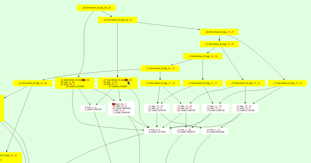
The result is on top, every node points to its arguments. The min and max
operations form a kind of "spine" of the expression tree, because they are
unions and intersection in the constructive solid geometry sense.
I also wrote a function to visualize the octree recursion itself, the output looks like this:

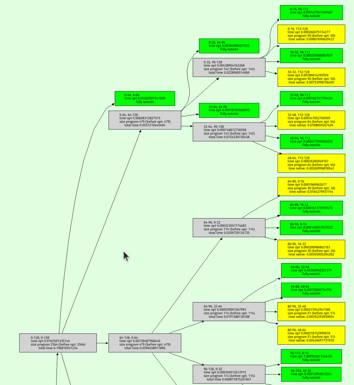
Green nodes are where the interval analysis determined that the output must be entirely outside the shape. Yellow nodes are where the octree recursion bottomed out.
C implementation
To achieve even faster performance, I decided to rewrite the implementation in C. While RPython is great for prototyping, it can be challenging to control low-level aspects of the code. The rewrite in C allowed me to experiment with several techniques I had been curious about:
-
musttailoptimization for the interpreter. - SIMD (Single Instruction, Multiple Data): Using Clang's
ext_vector_type, I process eight pixels at once using AVX (or some other SIMD magic that I don't properly understand). - Efficient struct packing: I packed the operations struct into just 8 bytes by limiting the maximum number of operations to 65,536, with the idea of making the optimizer faster.
I didn't rigorously study the performance impact of each of these techniques individually, so it's possible that some of them might not have contributed significantly. However, the rewrite was a fun exercise for me to explore these techniques. The code can be found here.
Testing the C implementation
At various points I had bugs in the C implementation, leading to a fun glitchy version of prospero:

To find these bugs, I used the same random testing approach as in the
RPython version. I generated random input programs as strings in Python and
checked that the output of the C implementation was equivalent to the output of
the RPython implementation (simply by calling out to the shell and reading the
generated image, then comparing pixels). This helped ensure that the C
implementation was
correct and didn't introduce any bugs. It was surprisingly tricky to get this
right, for reasons that I didn't expect. At lot of them are related to the fact
that in C I used float and Python uses double for its (Python) float
type. This made the random tester find weird floating point corner cases where
rounding behaviour between the widths was different.
I solved those by using double in C when running the random tests by means of
an IFDEF.
It's super fun to watch the random program generator produce random images, here are a few:
Performance
Some very rough performance results on my laptop (an AMD Ryzen 7 PRO 7840U with
32 GiB RAM running Ubuntu 24.04), comparing the RPython version, the C version
(with and without demanded info), and Fidget (in vm mode, its JIT made things
worse for me), both for 1024x1024 and 4096x4096 images:
| Implementation | 1024x1024 | 4096x4096 |
|---|---|---|
| RPython | 26.8ms | 75.0ms |
| C (no demanded info) | 24.5ms | 45.0ms |
| C (demanded info) | 18.0ms | 37.0ms |
| Fidget | 10.8ms | 57.8ms |
The demanded info seem to help quite a bit, which was nice to see.
Conclusion
That's it! I had lots of fun with the challenge and have a whole bunch of other ideas I want to try out, thanks Matt for this interesting puzzle.
PyPy v7.3.19 release
PyPy v7.3.19: release of python 2.7, 3.10 and 3.11 beta
The PyPy team is proud to release version 7.3.19 of PyPy. This is primarily a bug-fix release fixing JIT-related problems and follows quickly on the heels of the previous release on Feb 6, 2025.
This release includes a python 3.11 interpreter. There were bugs in the first beta that could prevent its wider use, so we are continuing to call this release "beta". In the next release we will drop 3.10 and remove the "beta" label.
The release includes three different interpreters:
PyPy2.7, which is an interpreter supporting the syntax and the features of Python 2.7 including the stdlib for CPython 2.7.18+ (the
+is for backported security updates)PyPy3.10, which is an interpreter supporting the syntax and the features of Python 3.10, including the stdlib for CPython 3.10.16.
PyPy3.11, which is an interpreter supporting the syntax and the features of Python 3.11, including the stdlib for CPython 3.11.11.
The interpreters are based on much the same codebase, thus the triple release. This is a micro release, all APIs are compatible with the other 7.3 releases. It follows after 7.3.17 release on August 28, 2024.
We recommend updating. You can find links to download the releases here:
We would like to thank our donors for the continued support of the PyPy project. If PyPy is not quite good enough for your needs, we are available for direct consulting work. If PyPy is helping you out, we would love to hear about it and encourage submissions to our blog via a pull request to https://github.com/pypy/pypy.org
We would also like to thank our contributors and encourage new people to join the project. PyPy has many layers and we need help with all of them: bug fixes, PyPy and RPython documentation improvements, or general help with making RPython's JIT even better.
If you are a python library maintainer and use C-extensions, please consider making a HPy / CFFI / cppyy version of your library that would be performant on PyPy. In any case, both cibuildwheel and the multibuild system support building wheels for PyPy.
What is PyPy?
PyPy is a Python interpreter, a drop-in replacement for CPython It's fast (PyPy and CPython performance comparison) due to its integrated tracing JIT compiler.
We also welcome developers of other dynamic languages to see what RPython can do for them.
We provide binary builds for:
x86 machines on most common operating systems (Linux 32/64 bits, Mac OS 64 bits, Windows 64 bits)
64-bit ARM machines running Linux (
aarch64) and macos (macos_arm64).
PyPy supports Windows 32-bit, Linux PPC64 big- and little-endian, Linux ARM 32 bit, RISC-V RV64IMAFD Linux, and s390x Linux but does not release binaries. Please reach out to us if you wish to sponsor binary releases for those platforms. Downstream packagers provide binary builds for debian, Fedora, conda, OpenBSD, FreeBSD, Gentoo, and more.
What else is new?
For more information about the 7.3.19 release, see the full changelog.
Please update, and continue to help us make pypy better.
Cheers, The PyPy Team